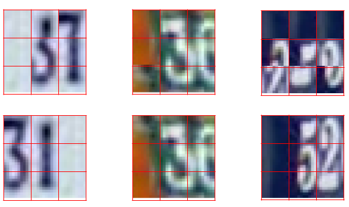
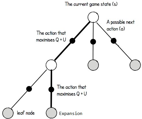
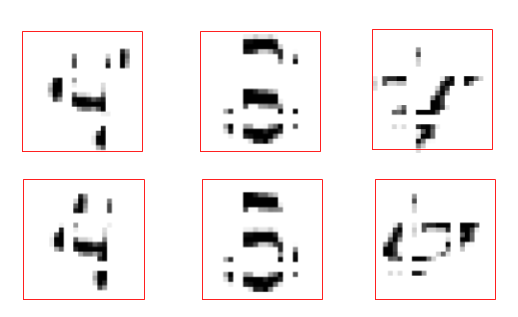
Puzzle Reassembly: Which row has been generated by our method?
The figure is composed of reassemblies coming from the MNIST SVHN dataset. The top row has been generated through our method (specifically selected pathological cases) and the bottom row is built from the ground truth.
Puzzle Reassembly using Model Based Reinforcement Learning
Abstract
In this paper, we are interested in solving visual jigsaw puzzles in a context where we cannot rely on boundary information. Thus, we train a deep reinforcement learning model that iteratively select a new piece from the set of unused pieces and place it on the current resolution. The pieces selection and placement is based on deep visual features that are trained end-to-end. Our contributions are twofold: First, we show that combining a Monte Carlo Tree Search with the reinforcement learning allows the system to converge more easily in the case of supervised learning. Second, we tackle the case where we want to reassemble puzzles without having a groundtruth to perform supervised training. In that case, we propose an adversarial training of the value estimator and we show it can obtain results comparable to supervised training.
Introduction
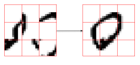
The focus of this paper is the reassembly of jigsaw puzzles. Our puzzles are made from 2D images and divided in 9 same-sized squared fragments, while also considering an erosion between each fragment. The problem consists in finding the optimal absolute position of each fragment on the reassembly. Moreover, we want to find this set of optimal positions using, on the one hand an iterative process, and one the other hand a content-based pattern matching method.
During the last decade, deep convolutional architectures as become the norm in most pattern matching tasks involving 2D images. Therefore, we choose to use such methods in order to extract semantic information from fragments and the reassembly. We build on the method proposed by Paumard et al.
In order to solve this problem, we construct this one as a Markov Decision Process, in order to solve it with a reinforcement learning (RL) algorithm. We build on the ExIt framework proposed by Anthony et al.
Our contributions are the following. First, a model based RL technique using a Monte Carlos Tree Search to compute simulations and two Neural Networks guiding the search and evaluating each final search's trajectory. And second, a variant using an adversarial training of the value estimator, allowing to tackle the case where we want to reassemble puzzles without having a groundtruth to perform supervised training.
Problem formulation and formalism
From a set of fragments coming from the same image, we want to solve their best reassembly by assigning each fragment to its optimal position.
Data representation
We want to introduce the notation of our data. is the number of fragments of a puzzle. is a flatten representation of the fragment given. is a special fragment filled with zeros. is a puzzle reassembly (a n-sized vector of fragments). is the optimal puzzle reassembly.
Goal, MDP and objective maximisation
Our goal being to find the optimal puzzle reassembly . We want to consider this problem as a Markov Decision Process (MDP) in order to solve it with a reinforcement learning algorithm. Starting from an initial state , we want to assign each fragment to its optimal position by taking the optimal actions . More specifically, we want to find one optimal policy in order to find those optimal actions.
We define the notation part of the MDP formalism: is the state at step defined by the tuple . With the puzzle reassembly at step . an n-sized vector, padded, of every fragment not used in .
The initial state drawn from the start-state distribution
An action is characterized by a fragment-position pair . With a fragment from and a unassigned position of the reassembly .
An action may be applied to a state using a deterministic transition function
A trajectory , is a sequence of states and actions
is the finite-horizon undiscounted return of a trajectory
The ExIt framework
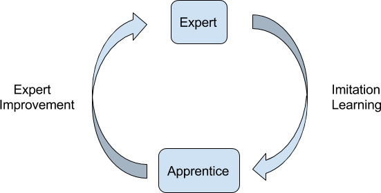
Human reasoning consists of two different kinds of thinking. When learning to complete a challenging planning task, such as solving a puzzle, humans exploit both processes: strong intuitions allow for more effective analytic reasoning by rapidly testing promising actions. Repeated deep study gradually improves intuitions. Stronger intuitions feedback to stronger analysis, creating a closed learning loop. In other words, humans learn by thinking fast and slow.
Overview: how does our method work?
The goal of this method is to find the optimal policy able to solve any puzzles from a specific dataset. In order, to achieve this goal we need to train a Reinforcement Learning (RL) algorithm able to find such policy.
We use a model based RL algorithm instead of less sample efficient algorithm such as Policy Gradients
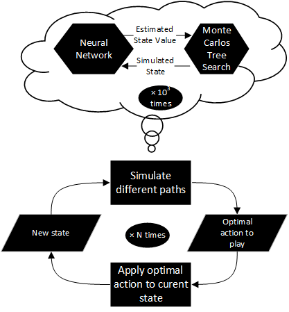
First, those fragments constitute the initial state.
Second, a "dreaming phase" occurs with the MCTS simulating multiple trajectories (of paths) and the networks estimating their action-state values. After its dream, the MCTS should give us a strong estimated of the optimal action.
Third, the transition function apply the optimal action on the actual state, giving us a new state. Again, this process is repeated until all fragments are assigned.
A first neural network, the Policy Network (PN) acts as the apprentice and try to mimic the expert policy . Thus, after training the PN generates an apprentice policy , such that:
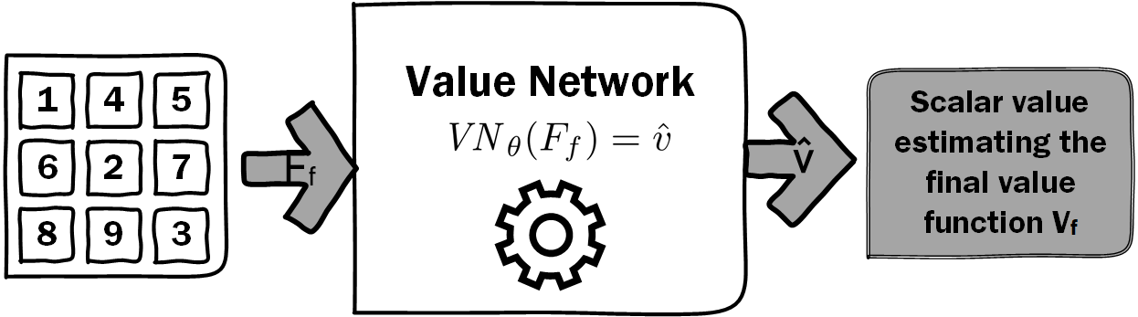
A second neural network, the Value Network (VN) acts as a Final Value Function () approximator. This VN approximate the finite-horizon return of the trajectory used to be in the final state . Therefore, it evaluates the quality of a complete reassembly.
During the Expert Improvement phase we use the PN to direct the MCTS toward promising moves, while effectively reducing the branching factor. In this way, we bootstrap the knowledge acquired by Imitation Learning back into the planning algorithm. In addition, after each simulation we backpropagate finals state value estimated by the VN. Indeed, this let our algorithm solve puzzles without having access to the ground truth after training.
Monte Carlo Tree Search
Monte Carlo Tree Search (MCTS) is an any-time best-first tree-search algorithm. It uses repeated game simulations to estimate the value of states, and expands the tree further in more promising lines. When all simulations are complete, the most explored move is taken.
The search
Each search, consist of a series of simulated games by the MCTS that traverse a tree from root state until a final state is reached. Each simulation proceeds in four parts.
We describe here the MCTS algorithm used for our method; further details can be found in the pseudocode bellow.
The MCTS is a tree search where each node corresponds to a state-action pair composed of a set of statistics,
is the mean value of the next state and a function that increases if an action hasn't been explored much or if the prior probability of the action is high:
Then, we expand the tree by initialising each legal child node with a softmax normalisation
Finally, when the rollout is complete, we compute
Exploration versus exploitation trade-off
On-line decision making involves a fundamental choice; exploration, where we gather more information that might lead us to better decisions in the future or exploitation, where we make the best decision given current information in order to optimize our present reward. This exploration-exploitation trade-off comes up because we're learning online. We're gathering data as we go, and the actions that we take affects the data that we see, and so sometimes it’s worth to take different actions to get new data.
In order to explore our synthetic environment and not only acting greedily, we use three kinds of exploration processes : an Upper Confident Bound
With: .
Pseudocode of our search algorithm
Functions approximators
In this method we use two Neural Networks working as functions approximators, the Policy Network (PN) and the Value Network (VN). In particular, the PN compute an estimation of the expert policy . Whereas, the VN estimate the Final Value Function, learning from the ground truth.
Value Network architecture
We use a problem dependent neural network architecture , with parameters . This neural network takes the final reassembly as input and output a scalar value estimating the finite-horizon return of the state's trajectory.
Policy Network architecture
The Policy Network , takes a state as input and outputs a move probability with components for each action .
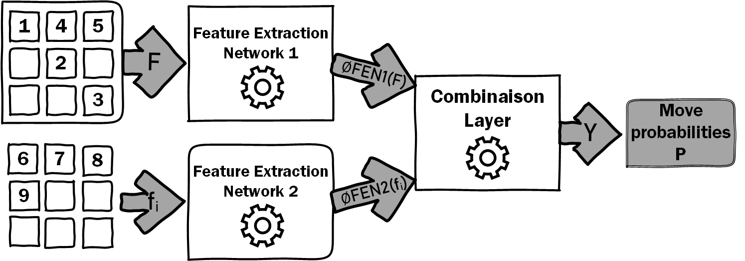
More specifically, the PN takes and the couple composing the state as separated inputs. On the one hand, the reassembly representation is extracted using a first Feature Extraction Network (FEN1). On the other hand, each individual fragment representation of is extracted using a second Feature Extraction Network (FEN2), with shared weights. Both FEN architecture is either, depending on the image complexity: a fully connected network or a deep convolutional architecture followed by a fully connected classifier.
The features of each FEN are then combined through a Combination Layer (CL). We use a bilinear product in order to optimally capture the spacial covariances among the features. In particular, we use this bilinear layer:
With, and the output of the first and second FEN respectively inside the ensemble and ; is a learnable tensor, such that , the number of positions in the puzzle; is the output of the CL, such that .
Finally, we flatten the output of the CL such as , with an action and we apply a softmax normalization
Training
Our algorithm learns these move probabilities and value estimates entirely from self-play; these are then used to guide its search for future reassembly.
At the end of each reassembly, the final reassembly is scored according to the cumulative reward of the environment . The VN parameters are updated to minimize the error between the predicted outcome and the environment outcome. While the PN parameters are updated to maximize the similarity of the move probabilities vectors to the search probabilities . Specifically, the parameters are adjusted by gradient descent with a mean-squared error for the VN loss and a cross-entropy for the PN loss.
Puzzle reassembly using Reinforcement Learning with discriminative value estimation
In this section, we will present a variant of our algorithm that doesn't need to have access to the ground truth during training (the optimal reassembly). This variant is inspired from the concept of discriminative value estimation for puzzle reassembly, introduced by Loïc Bachelot in an unpublished paper. In a first time, this concept will be summarized and in a second time our variant will be introduced.
Discriminative value estimation
This method can be seen as a mixture between an Actor-Critic
This discriminative-based technique is promising because it can be trained without having access to the ground truth, but it doesn't perform very well compared to a deep learning classifier baseline.
Our variant
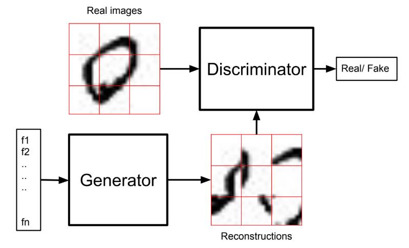
We merged the concept of discriminative value estimation to our previous method. Instead of the Value Network (VN), we replace this one with the discriminator network described above. The network architecture of the discriminator is the same as the VN architecture. The discriminator is trained (relatively) in the same way: by trying to classify where the reassembly comes from: from real images or generated by our algorithm?
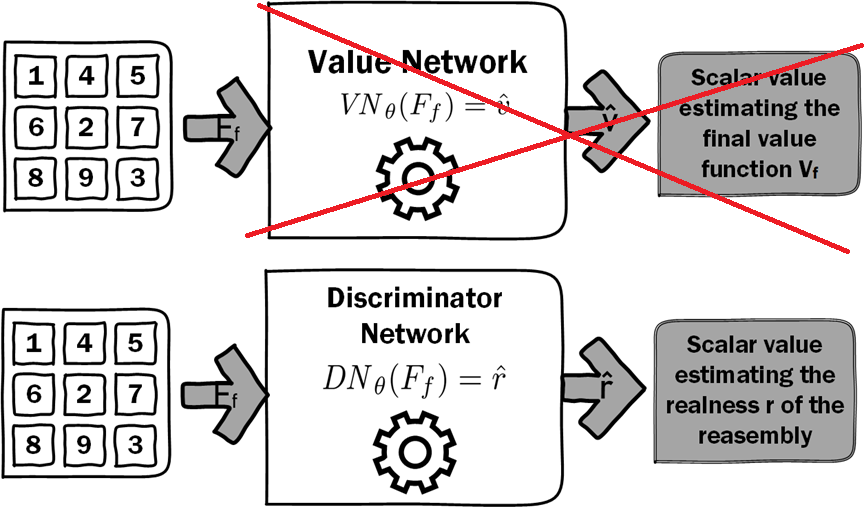
Since we don't have value estimated by the VN we directly use the probability estimated by the discrimator network. Therefore, instead of estimating the cumulative reward of the trajectory, we try to estimate the realness of the reassembly.
The goal of this merged version is to keep the best of both worlds. On the one hand, the reassembly look-ahead of the Monte Carlo Tree Search, on the other hand, the "unsupervised" setup of the discriminator value.
Experiments
We tested our methods for different kinds of datasets with different setups. First, we present the results of the MNIST dataset, second we consider an erosion of the MNIST images, then on the MNIST SVHN dataset and finally we present some preliminary results on a high resolution dataset. Two metrics are used in order to evaluate our methods. On the one hand, the fragments accuracy is the percentage of perfectly position fragments, on the other hand, the perfect reconstruction is a pixel-wise difference with the original image with a 10-pixel threshold. Experiments have been performed on a standard deskop machine without any kind of dedicated GPU.
MNIST
We tested on the MNIST dataset because the images are small enough for us to train the complete network and search for relevant hyper-parameters.
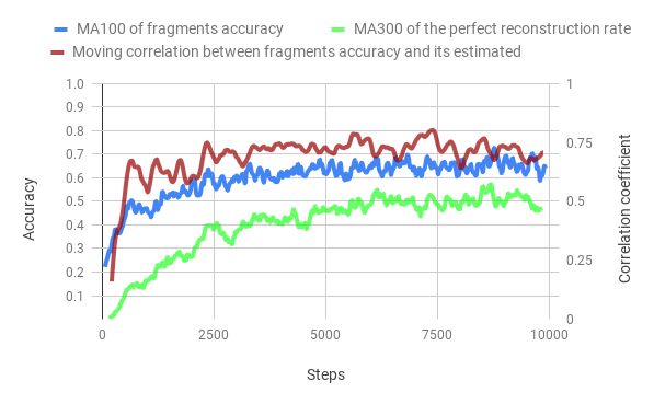
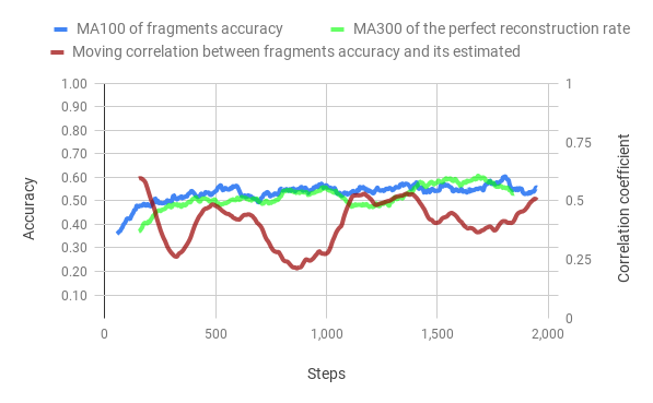
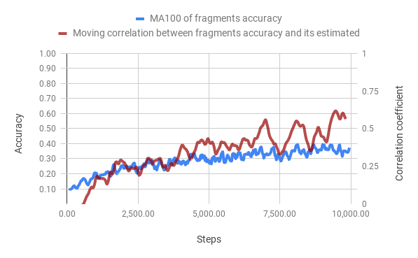
Evolution of the performance metrics throught training
In figures bellow, we can observe the evolution of accuracy thought the training of both methods. The training time of the merged method is 5 times smaller than the classic method. However, the correlation of the Value Network to the fragments accuracy is a lot stronger than the Discriminator Network, we train the VN to directly estimate this value so this not a surprise.
Influence of the number of simulations after training on the performance
In the figure bellow, we can see that the increase in the number of simulation increase logarithmically the accuracy. Also, both the classic method and the merged method give similar results, however, if the number of simulations is too low the merged method's accuracy is dropping. It may seem surprising that the merged method works so well without having access to the ground truth during the training phase.

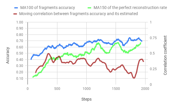
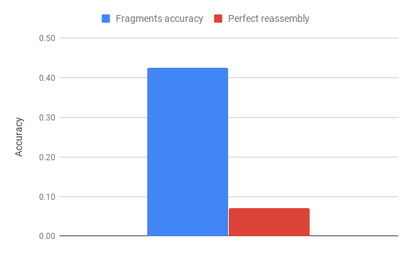
Merged method on eroded fragments
We decided to test our merged method using erosion between fragments (more than 10% of the image).
The test time result is really good , especially on the perfect reassembly metrics. During the training we observe both accuracy being more or less equal, while the correlation coefficient is not in the best shape ever.
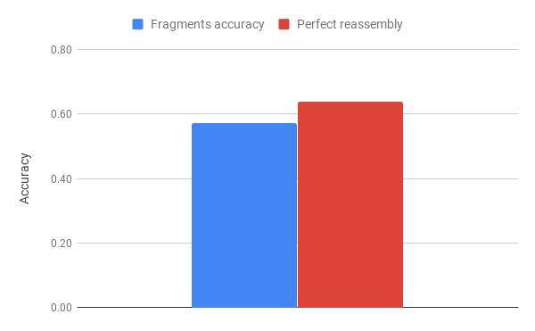
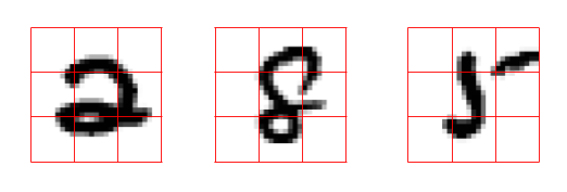
MNIST SVHN
After playing around with MNIST, we wanted to go further on the image complexity. Therefore we try our methods on MNIST SVHN, bellow some promising reconstructions.
On this dataset, with a really short training time (the accuract kept going up, but we had to cut the experiment), we achieve high fragments accuracy.
Car dataset
Looking forward to testing our method on a dataset with high resolution images, we did some quick training onto a car dataset using a VGG16 pre-trained on ImageNet as a feature extractor.
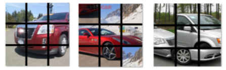
Our method did show some promising reconstructions, nonetheless the training time was really too short given the compute availaible. We achive 20% accuracy for the well positioned framents and a few perfect reassembly, that is still better that random and therefore show that our method should work with more time and compute available.
Related Work
Our project was inspired by several research articles which aim at solving this very problem using such techniques as deep learning. Other articles were unrelated to our purpose, but we adapted techniques described in there for our project purpose.
Review of puzzle solving methods
Most publications of this field
Without being interested in jigsaw puzzle solving, Doersch et al. proposed a deep neural network to predict the relative position of two adjacent fragments in
However, Paumard et al. in

First, they use deep learning in order to extract important features of each image fragments.
Then, they compare each couple of fragments features to predict the relative position of the two tiles, through a classifier.
Finally, they solve the best reassembly by computing the shortest path problem given the relative positions of each couples provided.
More specifically, the model perform quite well when we give it only the 9 accurate fragments. However, if we try to delete or to add outsider fragments to the puzzle, the accuracy decrease strongly. Furthermore, the increase of computation time is reasonable as long as the puzzle still contains 9 pieces, but any increment of the number of pieces leads to an factorial increase of the number of solution. Thus, the reassembly problem is NP-hard and the problem become quickly intractable.
MCTS based methods
As we seen, STOA methods like
More specifically, we are looking to use a similar approch as
Here we propose to used a deep reinforcement learning algorithm such as Alpha Zero
Instead of a handcrafted evaluation function and move-ordering heuristics, AlphaZero uses a deep neural network. This neural network takes the board position as an input and outputs a vector of move probabilities and a scalar value estimating the expected outcome of the game from position. AlphaZero learns these move probabilities and value estimates entirely from self-play; these are then used to guide its search in future games. Additionally, AlphaZero uses a general purpose Monte Carlo tree search (MCTS) algorithm
Acknowledgements
I would like to thank my Master's advisor David Picard for his invaluable help during this project. Additionally, I would like to thank Marie-Morgane Paumard and Loïc Bachelot for explaining their works.
This article was prepared using the Distill template and especially this modified version from the authors of Learning to Predict Without Looking Ahead: World Models Without Forward Prediction.
Citation
For attribution in academic contexts, please cite this work as
Johan Gras,

"Puzzle Reassembly using Model Based Reinforcement Learning", 2019.
BibTeX citation
@article{modelbasedrlpuzzlereassembly2019,
  author = {Johan Gras},
  title  = {Puzzle Reassembly using Model Based Reinforcement Learning},
  url    = {https://johan-gras.github.io/projects/puzzlereassembly/},
  note   = "\url{https://johan-gras.github.io/projects/puzzlereassembly/}",
  year   = {2019}
}
Open Source Code
Our code is not yet release, will be there soon!